Ever since I started studying atmospheric physics I was fascinated with the concept of chaos theory. The idea that even in a deterministical system (as long as it is non-linear) the smallest of deviations to the initial conditions can lead to unforeseen consequences is captivating.
Deep Neural networks are a fascinating topic in its own right. Not only because of their amazing capabilities in modern AI reseach, but also more fundamentally because of the universal approximation theorem. Where neural networks are universal function approximators, recurrent neural networks can be seen as universal dynamical system approximators. Since that means you can learn an arbitrary dynamical system just from data it suddenly becomes something incredibly useful for all kinds of scientific questions. For example you can parameterize a process that you don’t understand, but have lots of measurements of.
I wanted to demo this approach and chose a simple RNN to approximate the famous Lorenz ’63 dynamical system.
First we need to define the system itself that is governed by the differential equations; here I defined it as a torch nn.module to make use of the accelerated matrix multiplications.
# lorenz system dynamics
class Lorenz(nn.Module):
    """
    chaotic lorenz system
    """
    def __init__(self):
        super(Lorenz, self).__init__()
        self.lin = nn.Linear(5, 3, bias=False)
        W = torch.tensor([[-10., 10., 0., 0., 0.],
                          [28., -1., 0., -1., 0.],
                          [0., 0., -8. / 3., 0., 1.]])
        self.lin.weight = nn.Parameter(W)

    def forward(self, t, x):
        y = y = torch.ones([1, 5]).to(device)
        y[0][0] = x[0][0]
        y[0][1] = x[0][1]
        y[0][2] = x[0][2]
        y[0][3] = x[0][0] * x[0][2]
        y[0][4] = x[0][0] * x[0][1]
        return self.lin(y)
We then use a Runge-Kutta fourth order scheme to basically get a ground truth by integrating the differential equations starting from an initial condition y_0.
So far so good, we have a dynamical system and we are integrating it over time. This ground truth will become our training data for the neural network. In fact we will give some predefined context to the network and ask it to predict the next state of the system. Since we have the data from the ground truth we automatically have our “labels”. The neural network for this simple exercise is quite basic and looks like this:
class fcRNN(nn.Module):
    def __init__(self, input_size, hidden_dim, output_size, n_layers):
        super(fcRNN, self).__init__()
        self.hidden_dim = hidden_dim
        self.n_layers = n_layers
        self.rnn = nn.RNN(input_size,
                  		hidden_dim, n_layers,
                  		nonlinearity='relu',
                  		batch_first=True) # RNN hidden units
        self.fc = nn.Linear(hidden_dim, output_size) # output layer

    def forward(self, x):
        bs, _, _ = x.shape
        h0 = torch.zeros(self.n_layers,
            bs, self.hidden_dim).requires_grad_().to(device)
        out, hidden = self.rnn(x, h0.detach())
        out = out.view(bs, -1, self.hidden_dim)
        out = self.fc(out)
        return out[:, -1, :]
I put a link to my github gist at the end of the post, but for now let’s look at some of the results. The first one is an animation of training progress for 5000 epochs over time. The scatter plot shows the previously calculated ground truth. The network gets the first 15 time steps as a contest and is then tasked to predict the whole trajectory from there. What you can see is that in the beginning the network fails to correctly represent the system, but over time it becomes more stable and more similar to the ground truth. Keep in mind that exactly fitting all of the scatter points is incredibly difficult due to the “butterfly effect”. If you are only slightly incorrect at one of the previous timesteps the consequences can become arbitrarily large over time.
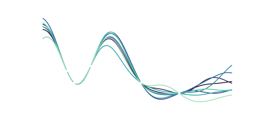
The second animation shows you all of the generated trajectories over the course of training, where early models are depicted in dark colors and late models in bright ones. Here it is quite cool to see that the first two models really didn’t yet train enough to capture the system’s dynamics and immediately leave the trajectory once the 15 context samples ran out. From there you can observe that models that have trained for longer better approximate the true state shown in blue. Now again after one loop or so the even the trained models diverge due to minor differences at some point in the past, but it is worth noting, that the trained recurrent networks (especially the ones with more training time) correctly characterize the dynamical system with its two lobes spanning the 3D space. Now what that means is that you can use the network to describe the system and you probably have a useful model when combined with some data fusion process like Kalman filtering.
Feel free to have a look at the full code and play around with the model yourself @github-gist.
 means that for any finite batch of function values
  , where
 ![\mathbf{f} = \left[ f(\mathbf{x_1}, ..., f(\mathbf{x_n}))\right] \sim \mathcal{N}(\mu, K)](https://www.markusernst.org/wp-content/ql-cache/quicklatex.com-eb4f409d8ec133a700fcfcfacc948440_l3.svg "Rendered by QuickLaTeX.com") holds.
holds.![\begin{equation*} \left[ {\begin{array}{c} f \\f^* \end{array} } \right] = \mathcal{N}\left( \mu, \left[ {\begin{array}{cc} K + \sigma^2 \mathbb{I}_n & K_* \\K_*^T & K_{**} \\ \end{array} } \right] \right). \end{equation*}](https://www.markusernst.org/wp-content/ql-cache/quicklatex.com-cb2057e43992e88a87091fb8df55e706_l3.svg "Rendered by QuickLaTeX.com")
 part at the top left in the kernel-matrix above.
 with
with  the lengthscale and
  the signal variance. But feel free to try out another kernels, like Brownian
  for example.
 and a variance
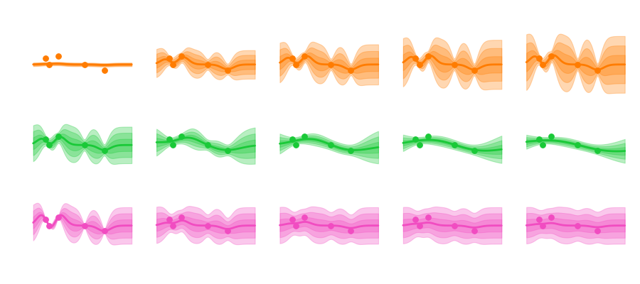
 with values
  ,
,  with noise in each point
  and points
  for which we want to predict the output, adapting our probability distribution leads to:
 , with


 and the noise that can influence how we model our data. Varying these parameters looks like this: